Page 346 - Process Modelling and Simulation With Finite Element Methods

Electrokinetic Flow 333

Surface: Y Arrow: velocity vectors !?
4 762
4 524
15 4 286
4 048
3 81
1 3 571
3 333
05 3 035
2 857
2 619
0 2 381
2 143
-0 5 1 905
1 667
1 429
-1 119
0 3524
-1 5 0 7143
0 4762
0 2381
-2
-2 -1 0 1 2 3 4 Min 0
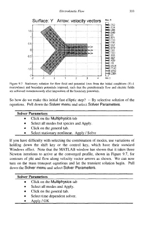
Figure 9.7 Stationary solution for flow field and potential lines from the initial conditions (Y=1
everywhere) and boundary potentials imposed, such that the pseudosteady flow and electric fields
are achieved instantaneously after imposition of the boundary potentials.
So how do we make this initial fast elliptic step? -- By selective solution of the
equations. Pull down the Solver menu and select Solver Parameters.
Solver Parameters
0 Click on the Multiphysics tab
0 Select all modes but species and Apply.
0 Click on the general tab.
Select stationary nonlinear. Apply / Solve

If you have difficulty with selecting the combination of modes, use variations of
holding down the shift key or the control key, which have their standard
Windows effect. Note that the MATLAB window has shown that it takes three
Newton iterations to arrive at the converged profile, shown in Figure 9.7, for
contours of phi and flow along velocity vector arrows as shown. We can now
turn on the mass transport equations and let the transient solution begin. Pull
down the Solver menu and select Solver Parameters.

Solver Parameters
Click on the Multiphysics tab
0 Select all modes and Apply.
0 Click on the general tab.
0 Select time dependent solver.
Apply/OK