Page 351 - Process Modelling and Simulation With Finite Element Methods

338 Process Modelling and Simulation with Finite Element Methods

As before, we need to stage our solution to set up the pseudosteady velocity and
potential fields initially, then turn on the species transport.

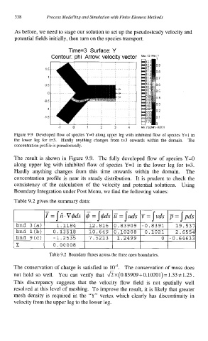
Time=3 Surface: Y
Contour: phi Arrow: velocity vector

15
1
05
0
05
1
15
1 0 1 2 3 4 Mm752Mm00131
Figure 9 9 Developed flow of species Y=O along upper leg with inhibited flow of species Y=l in
the lower leg for t=3. Hardly anything changes from t=3 onwards within the domain. The
concentration profile IS pseudosteady.

The result is shown in Figure 9.9. The fully developed flow of species Y=O
along upper leg with inhibited flow of species Y=l in the lower leg for t=3.
Hardly anything changes from this time onwards within the domain. The
concentration profile is near its steady distribution. It is prudent to check the
consistency of the calculation of the velocity and potential solutions. Using
Boundary Integration under Post Menu, we find the following values:

Table 9.2 gives the summary data:

Table 9.2 Boundary fluxes across the three open boundaries.
The conservation of charge is satisfied to The conservation of mass does
not hold so well. You can verify that ~~(0.83909+0.10201)=1.33#1.25.
This discrepancy suggests that the velocity flow field is not spatially well
resolved at this level of meshing. To improve the result, it is likely that greater
mesh density is required in the “Y” vertex which clearly has discontinuity in
velocity from the upper leg to the lower leg.