Page 349 - Process Modelling and Simulation With Finite Element Methods

336 Process Modelling and Simulation with Finite Element Methods

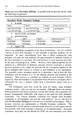
menu and select Boundary Settings. In parallel with the previous set up, make
the following assignments:

Boundary Mode I Boundary Settings

bnd 1 bnd 3 bnd 9 bnd 2,4,5,6,7,8
u=0.707 107*Qb u=0.707 107*Qa u=Qc unchanged
v=0.707107*Qb v=-0.707107*Qa v=o
species mode: unchanged
potential mode
bnd 1 I bnd3 I bnd9 I bnd 2,4,5,6,7,8
Neumann I Neumann I Neumann 1 unchanged
I G=Ib/sigr I G=Ia/sigr I G=Ic/sigr
ADDIv/OK
0
There is an underlying assumption in the above formulation. Use of a uniform
velocity at each flow boundary is only possible if pressure gradient can be
neglected. In 'pure' electrokinetic flow, that is where conductivity, zeta
potential, viscosity are each uniform, the approximation of uniform velocity at
the flow boundaries is excellent. The total pressure in each reservoir must also
be the same (Cummings et al., 2000). However, when liquid properties are not
uniform or a differential of dynamics pressure between reservoirs is present,
pressure gradients arise within the network and the assumption implicit in the
above treatment that velocity is uniform at each boundary is not appropriate.
The generally correct treatment would be to determine I and Q from the flow
boundaries and use relation 9.11 for the uniform pressure and potential at the
boundary. That pressure or potential are uniform at each boundary follows
rigorously when the boundary is at a position where the flow is developed, that is
sufficiently far (say, a channel width) from a disturbance region such as a
junction.
The formulation used does avoid the need for further weak boundary
constraint modes - only wcu and wcv are needed. Although there is an analogy
between pressure and electric potential, current and velocity, these quantities are
treated fundamentally differently with regard to the need for weak boundary
constraints. The velocity boundary conditions now require weak boundary
constraints on all boundaries (not just the wall surfaces). So we will need to
alter the Boundary Settings for wcu and wcv to include all boundaries. This is
because velocities are implemented as Dirichlet boundary conditions. The
Neumann BCs for the current in potential mode, however, do not require and are
incompatible with weak boundary constraints as we learned earlier. Neumann
conditions, since they are the default for FEM, are non-constraints even when