Page 343 - Process Modelling and Simulation With Finite Element Methods

330 Process Modelling and Simulation with Finite Element Methods

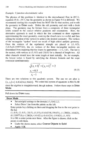
Example: Y-junction electrokinetic valve
The physics of this problem is identical to the microchannel flow in $9.3.1,
equation (9.4)-(9.7), but the geometry as shown in Figure 9.6 is different. We
recommend starting this example from the MAT-file for that section, and to edit
the geometry in Draw mode. Delete the old geometry and start with a fresh
plane. The geometry may be formed from a composite of three rectangular
solids rotated to the correct relative positions and orientations. Here, the
alternative approach is used in which the line command to draw segments
approximating the exact geometry, coercing the closed curve to a solid, and then
editing the location of the vertices to achieve the desired symmetry. The vertices
of the rectangular “spokes” taxed our recall of high school analytic geometry.
Once the vertices of the equilateral triangle are placed at {(1,-0.5),
(1,0.5),(0.133977,0)), the six vertices of the three rectangular sections are
determined from requiring that the slopes be appropriate - { + 1 ,-I ,0) , The last is
the easiest, with vertices at (3,-0.5) and (3,OS) for a channel of length two. All
other channels should have the same length at least initially. So, for example,
the lowest vertex is found by satisfying the distance formula and the slope
constraint simultaneously:

y1 +0.5 =I (9.13)
x, -1
There are two solutions to this quadratic system. The one we are after is
(3, y,) =(~.414214,1.91421). We coded this system of equations in MATLAB
since the algebra is straightforward, though tedious. Follow these steps in Draw
Mode:

Pull down the Draw menu.

Draw Mode
Set axidgrid settings to the domain [-3,3]x[-2,2].
Select Draw Line from the palette on the left.
Enter points buy clicking on them and dragging the line to the next point in
the list:
(l,-O.S), (3,-0.5), (3,0.5), (1,O.S),(-O.414214,1.91421), (-1.28024,1.41421),
(0.133977,0),(-1.28024,-1.41421),(-0.414214,-1.91421), (1 ,-0.5)
It is OK to enter points near these. After the figure is drawn, click on the
points to edit them.
Under the drawn menu, select Coerce Objects to Solid