Page 339 - Process Modelling and Simulation With Finite Element Methods

326 Process Modelling and Simulation with Finite Element Methods

Time=l Surface: Y
Contour: phi Arrow:Velocity vector Max 3 Max 1
n2
!
1 _I..... ... I... .............. ..I. ....... I...... ... ....... :.....2 09
...... .........
.:.
0 8 -~. .:. .:. ..... .......... ...... ..............
,;
:
08
0.6 -1.. .....................................................
07
06
05
04
03
-0.6 .;. ........ : ........ .........:... .................... 02
-0 8 {. ......... .: ... ...I.. ......... .!. ................. .:. ....... ;. ... - 01
-1 -:. .................. :.... .................. ;. ................. ..:
I I n
0 0.5 1 1.5 2 2.5 3 Min. 0 Min: -0.OC I1 03
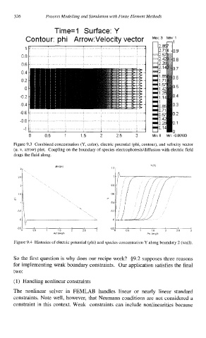
Figure 9.3 Combined concentration (Y, color), electric potential (phi, contour), and velocity vector
(u. v, arrow) plot. Coupling on the boundary of species electrophoresis/diffusion with electric field
drags the fluid along.

1
25 r
I
2 08
I
06
15-1 r
l.\ 04
,
02
05-1
0
Arc Lenglh Arc Length
Figure 9.4 Histories of electric potential (phi) and species concentration Y along boundary 2 (wall).

So the first question is why does our recipe work? 39.2 supposes three reasons
for implementing weak boundary constraints. Our application satisfies the final
two:
(1) Handling nonlinear constraints
The nonlinear solver in FEMLAB handles linear or nearly linear standard
constraints. Note well, however, that Neumann conditions are not considered a
constraint in this context. Weak constraints can include nonlinearities because