Page 334 - Process Modelling and Simulation With Finite Element Methods

Electrokinetic Flow 321

the evolution of the front is then computed in time. The test problem is
two-dimensional and the channel width can be taken as 1 unit, with the length
equal to 6 units.
There are a number of distinct steps in problem complexity. (1) With the
parameter values suggested above, the electric field will be uniform and in the
direction of the channel. The concentration will move with a uniform flow with
the front thickening from diffusion. (2) Setting <, # 1 gives a non-uniform
wall zeta potential with walls exposed to full concentration of the computed
species having zeta potential <, and those exposed to zero concentration
< = - 1 , giving variation of slip boundary velocity through the first of boundary
conditions 9.4. The electric field remains uniform and in the channel direction,
but the velocity field will be altered. The concentration front will be modified
from the pure diffusion case by the non-uniform velocity field. (3) Setting
z = &I and p = 1 will introduce electrophoresis. The computed species will
translate in the channel direction in addition to being moved by the liquid
velocity. (4) Finally, setting Or # 1 introduces non-uniform electrical
conductivity. This leads to changes in the electric field associated with changes
in concentration (Y) so the electric field is no longer uniform or, where
concentration gradient is not everywhere in the direction of the channel, in the
channel direction.

Wa II

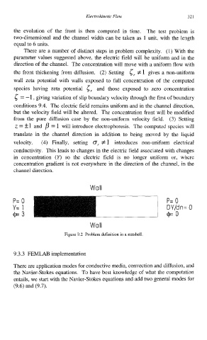
Wa II
Figure 9.2 Problem definition in a nutshell.

9.3.3 FEMLAB implementation

There are application modes for conductive media, convection and diffusion, and
the Navier-Stokes equations. To have best knowledge of what the computation
entails, we start with the Navier-Stokes equations and add two general modes for
(9.6) and (9.7).