Page 330 - Process Modelling and Simulation With Finite Element Methods

Electrokinetic Flow 311

Equation (9.1) defined the ideal dim constraint. So what is this? The analogous
contributions to the weak formulation are:

The derivative of the constraint function (h) is now missing from the second
contribution in (9.2). It is argued that (9.2) better “balances” the constraint
r(@)=O in the case when Y is nonlinear or contains derivatives of @, which are not
as accurately estimated by FEM for their contribution to h.

Now use the triangle on the toolbar (mesh) then select solve (=). ect.mat was a
linear problem, so the linear solver is the default. Ours computed so rapidly that
we did not notice the solution time. Enter post mode and compute the following:

Post Mode
Boundary integration: bnd 24,21,5,6 nx*phix+ny*phiy
Boundary integration: bnd 24,21,5,6 lm

Since writing Chapter 7, we have learned that nx and ny are symbols available
on the boundary to compute the components of the normal vector in the
coordinate directions. Thus the first calculation is equivalent to the standard
formula

(9.3)
dn
where the unit outward pointing normal is used. We did this “by hand” since we
had defined the normal vector as a constant, even though the sector boundary
was slightly curved in defining the geometry. Now refine the mesh using the
standard toolbar - inverted triangle in the triangle. Recompute the boundary
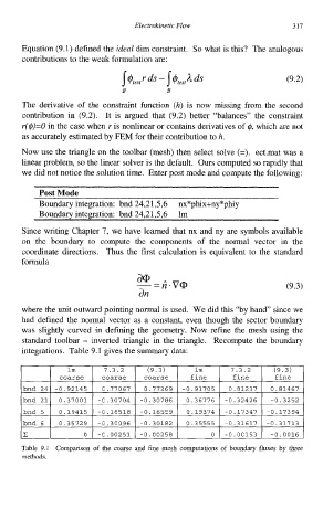
integrations. Table 9.1 gives the summary data:

Table 9.1 Comparison of the coarse and fine mesh computations of boundary fluxes by three
methods.