Page 327 - Process Modelling and Simulation With Finite Element Methods

314 Process Modelling and Simulation with Finite Element Methods

Thus, in preparation for our model, a simple example illustrating how weak
boundary constraints can be used, in this case to compute boundary fluxes more
accurately, is shown in $9.2, with the example drawn from the forward ECT
problem of 57.3.2. In section $9.3, our “building block” 2-D electrokinetic flow
model is set out.

9.2 Weak Boundary Constraints: Revisiting ECT

The FEMLAB 2.3 User’s Guide and Introduction [l] has an excellent section on
modeling approaches, including a discussion of weak boundary constraints. The
section gives three primary reasons for using weak boundary constraints:
Very accurate flux computations
Handling nonlinear constraints
Implementing constraints using derivatives.

In this section, we discuss how to use the weak boundary constraint to compute
fluxes very accurately.
Before we do this, we need to re-visit the role of Lagrange multipliers in
boundary and auxiliary constraint satisfaction through the finite element method.
This was done in its full glorious detail in $2.3.1. Now, if you have Neumann
boundary conditions, on a boundary B, then there is nothing to do - these are
naturally computed using the FEM weak formulation as described in Chapter 2.
You can think of Neumann conditions as being “neutral” in that unless you
specify a constraint, they happen by default. So we will put it here simplistically
that on a given boundary B we have a nonlinear constraint r(@)=O, where 4 is the
dependent variable. A second quantity that FEMLAB utilizes is h, which is the
derivative of the constraint, i.e. h=-r’(@). If there are more than one dependent
variable, then h is a vector valued quantity (the gradient). The simplest form that
can be taken for the constraint is a linear function: r(4)=Q0 - 4, which is the
Dirichlet condition. In this case, h=l. You might have been wondering for
some time about what h and r were in specifying Dirichlet conditions.
If you select the Dirichlet radio button in general mode (boundary setting),
for instance, specify r=l-phi (in general form, h is automatically computed by
symbolic differentiation), then FEMLAB implements ideal boundary conditions
for that boundary, which adds two more contributions to the weak formulation of
the problem. These are subsequently discretized by the Galerkin method on the
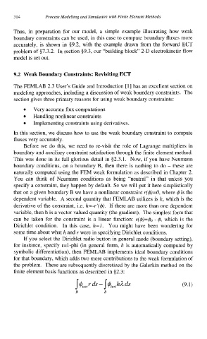
finite element basis functions as described in $2.3:

(9.1)