Page 337 - Process Modelling and Simulation With Finite Element Methods

324 Process Modelling and Simulation with Finite Element Methods

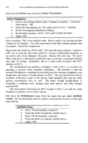
Pull down the Solver menu and select Solver Parameters.

Solver Parameters
0 Click on the Settings button under “Scaling of variables.” Check the
None option. OK
Select the timestepping tab. Set output times to 0:O.l: 1 (default)
Set the timestepping algorithm to fldaspk
Set absolute tolerance: u 0.01 v 0.01 p Inf Y 0.001 phi 0.001
0
Apply/OK
Now a warning. This is not going to work. Just to verify it, try solving and take
a break for five minutes. You will come back to find little solution progress has
been made. Cancel the computation.
Where does the model go off the rails? We tried the usual suspects - system is
stiff? So we tried the stiff solver (ode23s)! System is differential-algebraic, so
we tried a dae solver (fldaspk). No good. Reduce the time step. No good.
When reduced to a ridiculously small time step, we did get a converged solution
after ages of waiting. Remember, this is a small mesh (compare with ECT
problem in §9.2!).
We foreshadowed the problem in Chapter 7 and in 09.1, so no prizes for
guessing it involves weak boundary constraints. The problem is that the
standard Multiphysics couplings are not picking up the boundary couplings, even
though they are linear or pseudo-linear, in (9.4). The top and bottom velocity
boundary conditions couple to the electric field (gradient phi) and the outlet
species concentration does as well. The latter, though pseudo-linear, is
eventually a nonlinear term, feeding back both species and field strength
quadratically.
Our prescription, following the ECT example in $9.2, is to add two weak
boundary constraints; one for each velocity.
Pull down the Multiphysics menu from the menu bar and select Add/Edit
modes. We should already have ns, species, and potential in place on the right
hand side list.

Admdit Modes
Select “Weak boundary constraint”
Name the mode wcu and the variable lmu>>
Select “Weak boundary constraint”
Name the mode wcv and the variable lmv>>
0
Apply/OK