Page 87 - Process Modelling and Simulation With Finite Element Methods

14 Process Modelling and Simulation with Finite Element Methods

stationary solver. So we can only influence the transient solution with a
temperature dependent diffusivity. So change the initial condition to u(t0)=400,
i.e., the left boundary jumps to u=500 to define time z=O.
elements.”
Now pull down the Solve menu and select the Parameters option. This pops
up the Solver Parameters dialog window.

Solver Parameters
General tab: select time dependent
Jacobian: numeric
Time-stepping tab. Take output times 0:0.01:0.2
Solve
Cancel/OK
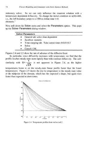
Figures 2.4 and 2.5 show the rate of advance of the diffusive front.
In particular, since diffusivity increases with temperature, we find that the
profile reaches steady state more rapidly than with constant diffusivity. The self-
v
n
similarity with q=- is not apparent in Figure 2.4, as the higher
JE
temperatures home in on the steady-state linear profile faster than the lower
temperatures. Figure 2.5 shows the rise in temperature to the steady state value
at the midpoint of the domain, which has the expected s-shape, but again rises
faster than expected at short times.

x poslllon
Figure 2.4 Temperature profiles from T=O to 2=0.2.