Page 93 - Process Modelling and Simulation With Finite Element Methods

80 Process Modelling and Simulation with Finite Element Methods

2r
1.75 1

1.25 1
0.75 li

0.25 1
i-,
,
,
I
,
2 4 6 8 10
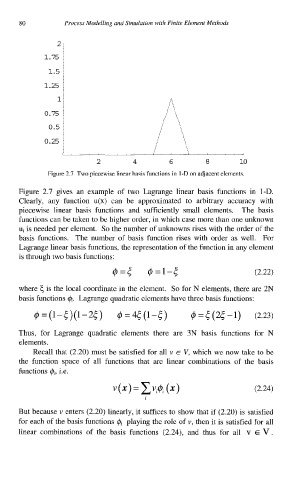
Figure 2.7 Two piecewise linear basis functions in 1-D on adjacent elements.
Figure 2.7 gives an example of two Lagrange linear basis functions in 1-D.
Clearly, any function u(x) can be approximated to arbitrary accuracy with
piecewise linear basis functions and sufficiently small elements. The basis
functions can be taken to be higher order, in which case more than one unknown
ui is needed per element. So the number of unknowns rises with the order of the
basis functions. The number of basis function rises with order as well. For
Lagrange linear basis functions, the representation of the function in any element
is through two basis functions:
@=( @=1-( (2.22)

where 5 is the local coordinate in the element. So for N elements, there are 2N
basis functions q$. Lagrange quadratic elements have three basis functions:
@=(1-<)(1-2<) @=4((1-() $=<(2(-1) (2.23)

Thus, for Lagrange quadratic elements there are 3N basis functions for N
elements.
Recall that (2.20) must be satisfied for all v E V, which we now take to be
the function space of all functions that are linear combinations of the basis
functions q$, i.e.

But because v enters (2.20) linearly, it suffices to show that if (2.20) is satisfied
for each of the basis functions @i playing the role of v, then it is satisfied for all
linear combinations of the basis functions (2.24), and thus for all v E V.