Page 94 - Process Modelling and Simulation With Finite Element Methods

Partial Differential Equations and the Finite Element Method 81

Thus, the condition (2.24) is equivalent to a system of (k+l)N equations [(2.20)
for each 4,] in (k+l)N unknowns (the u, ), where k is the order of the element
(k=l linear, k=2 quadratic, etc.).
Then there is the reason why FEM with FEMLAB has such utility.
FEMLAB automates the assembly of the (k+l)N equations (2.20). First, we note
that T(u) and F(u) are general, potentially nonlinear, functions of u. So, in
general, the solution is not achievable in closed form. In Chapter One, we
showed that FEMLAB has a built-in nonlinear solver for 0-D problems, i.e.
f(u)=O, where u was a single unknown value. The nonlinear solver was based on
Newton’s Method. The N-dimensional analogue of Newton’s Method for the
vector equation
L(U)=O (2.25)

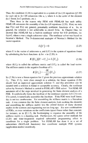
where U is the vector of unknowns u, and L(U) is the system of equations found
by substituting the basis functions 4, for v in (2.20), is

(2.26)

where K(Uo) is called the stiffness matrix and L(U0) is called the load vector.
The stiffness matrix is the negative Jacobian of L:
(2.27)

So (2.26) is now a linear equation for U given the previous approximate solution
Uo. Thus, if Uo were close enough to a solution, the linear equation (2.26)
should find an improved approximate solution U, and this procedure can be
iterated until a solution is found to acceptable accuracy. Clearly, the nonlinear
solver by Newton’s Method is central to FEMLAB’s PDE solver. Yet FEMLAB
automates all of the steps involved in generating the finite element analysis of a
PDE. It symbolically forms the Jacobian of the nonlinear operator L(U) if it can.
If it cannot, it numerically assembles the Jacobian. If the PDE were itself linear,
this is not too cumbersome. Yet assembling the stiffness matrix is a Herculean
task - it was common that the finite element analysis, both meshing the elements
and assembling the stiffness matrix was the central feature of many doctoral
studies in the sciences and engineering not too long ago. For new combinations
of PDEs, or even variations on the coefficients (quasi-linear rather than constant,
for instance, as in 42.1.2), the bookkeeping to organize the assembly of the
stiffness matrix is a daunting task. Furthermore, the sparse solver methods for
(2.26) and time-integration required substantial programming effort to
coordinate for a single problem. Yet FEMLAB has done it as a set of
subroutines (MATLAB functions) that coordinate multiple PDE systems
(application modes) seamlessly.