Page 99 - Process Modelling and Simulation With Finite Element Methods

86 Process Modelling and Simulation with Finite Element Methods

x D* x 8 ~ ~ ~ ~ ~ ~ ~ % ~ ~ ~ ~ ~ ~ ~ ~ ~ ~
0

-0.02

-0.04
-0.06

-0.08
h
X
v
a
-0.1
-0.12

4.14
-0.16

-0.18
X
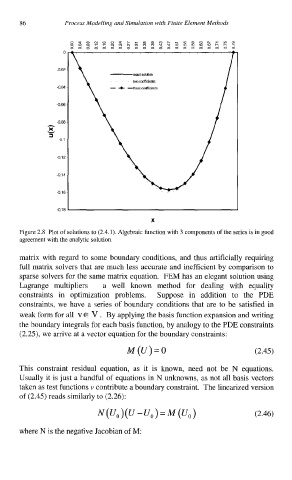
Figure 2.8 Plot of solutions to (2.4.1). Algebraic function with 3 components of the series is in good
agreement with the analytic solution.
matrix with regard to some boundary conditions, and thus artificially requiring
full matrix solvers that are much less accurate and inefficient by comparison to
sparse solvers for the same matrix equation. FEM has an elegant solution using
Lagrange multipliers - a well known method for dealing with equality
constraints in optimization problems. Suppose in addition to the PDE
constraints, we have a series of boundary conditions that are to be satisfied in
weak form for all v E v . By applying the basis function expansion and writing
the boundary integrals for each basis function, by analogy to the PDE constraints
(2.25), we arrive at a vector equation for the boundary constraints:
M(U)=O (2.45)

This constraint residual equation, as it is known, need not be N equations.
Usually it is just a handful of equations in N unknowns, as not all basis vectors
taken as test functions v contribute a boundary constraint. The linearized version
of (2.45) reads similarly to (2.26):

where N is the negative Jacobian of M: