Page 101 - Process Modelling and Simulation With Finite Element Methods

88 Process Modelling and Simulation with Finite Element Methods

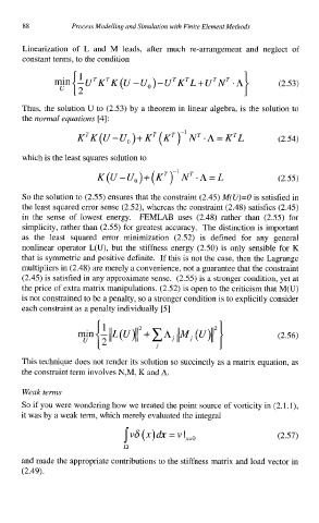
Linearization of L and M leads, after much re-arrangement and neglect of
constant terms, to the condition

(2.53)

Thus, the solution U to (2.53) by a theorem in linear algebra, is the solution to
the normal equations [4]:

K~K(U -u, >+ K~ (K' )' ivT .A = KTL (2.54)

which is the least squares solution to
K (U -u,,>+(K~ r1 N~ .A = L (2.55)

So the solution to (2.55) ensures that the constraint (2.45) M(U)=O is satisfied in
the least squared error sense (2.52), whereas the constraint (2.48) satisfies (2.45)
in the sense of lowest energy. FEMLAB uses (2.48) rather than (2.55) for
simplicity, rather than (2.55) for greatest accuracy. The distinction is important
as the least squared error minimization (2.52) is defined for any general
nonlinear operator L(U), but the stiffness energy (2.50) is only sensible for K
that is symmetric and positive definite. If this is not the case, then the Lagrange
multipliers in (2.48) are merely a convenience, not a guarantee that the constraint
(2.45) is satisfied in any approximate sense. (2.55) is a stronger condition, yet at
the price of extra matrix manipulations. (2.52) is open to the criticism that M(U)
is not constrained to be a penalty, so a stronger condition is to explicitly consider
each constraint as a penalty individually [5]

!- (2.56)

This technique does not render its solution so succinctly as a matrix equation, as
the constraint term involves N,M, K and A.

Weak terms
So if you were wondering how we treated the point source of vorticity in (2.1. l),
it was by a weak term, which merely evaluated the integral

jd (X)h = v Ixzo (2.57)
n
and made the appropriate contributions to the stiffness matrix and load vector in
(2.49).