Page 106 - Process Modelling and Simulation With Finite Element Methods

Partial Differential Equations and the Finite Element Method 93

If YOU observed closely, you could see that the cubic interpolation function
in Lagrange elements needs four nodes whereas in Hermite elements only two
nodes are required. Hermite elements are commonly used in solving load and
stress distributions of trusses.
Further to these two types, FEMLAB offers curved mesh elements and
Argyris elements. The curved mesh elements are provided to facilitate the
approximation of true boundaries with higher accuracy. The Argyris elements
are fifth order Hermite elements using nodal values as well as derivatives up to
second order. It also uses the normal components of vu at the midpoints of the
sides. Argyris elements require determination of 21 constants of a quintic
polynomial. In addition to predefined elements, FEMLAB allows user defined
elements. We advise interested readers to consult FEMLAB manuals for detailed
description on how to define a new class of elements.
Here we provided a sufficient description of basic elements to make a
beginner comfortable with the jargon and using the elements with some
understanding. With FEMLAB, one does not need to become an expert in
meshing techniques and development of elements. As you have already seen,
once you generate the domain over which the differential equations are to be
solved, meshing is just a click of a button away. However, if a reader is
interested in understanding the basic concepts, development of elements and
meshing techniques, refer to [6] and references there in.

Exercise:
To explain the formulation and solution methods involved in FEM, a worked
example is considered. In 1.5.1, heat transfer in a nonuniform medium was treated.
Here we consider similar problem with more simplifications. Instead of a variable
heat transfer coefficient, we consider a constant coefficient and considerxx) to be
uniform over the length of the domain. The length of the domain L=l. Figure 2.10
shows the physical system. We assume the heat flow across any cross section
(shown as A in Fig. 2.10) normal to the centre axis to be uniform. Therefore the
temperature varies only along the axis: hence reduced dimensionality.
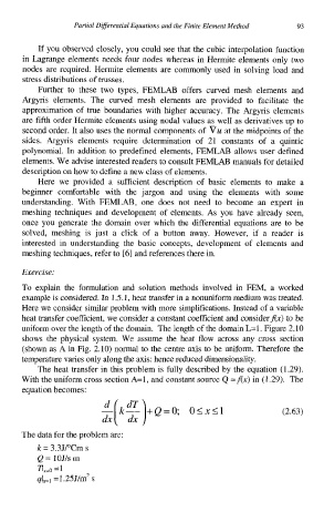
The heat transfer in this problem is fully described by the equation (1.29).
With the uniform cross section A=l, and constant source Q =f(x) in (1.29). The
equation becomes:
(2.63)

The data for the problem are:
k = 3.3J/"Cm s
Q = 1OJ/s m
n,, =I
qIG1 =1.25J/m2 s