Page 107 - Process Modelling and Simulation With Finite Element Methods

94 Process Modelling and Simulation with Finite Element Methods

I I
L
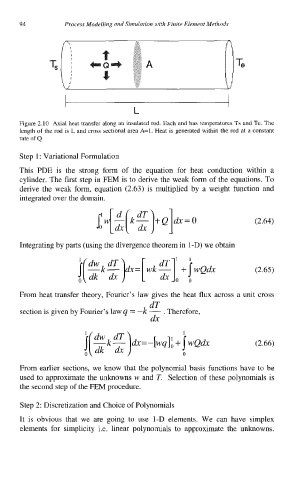
Figure 2.10 Axial heat transfer along an insulated rod. Each end has temperatures Ts and Te. The
length of the rod is L and cross sectional area A=l. Heat is generated within the rod at a constant
rate of Q.
Step 1: Variational Formulation

This PDE is the strong form of the equation for heat conduction within a
cylinder. The first step in FEM is to derive the weak form of the equations. To
derive the weak form, equation (2.63) is multiplied by a weight function and
integrated over the domain.

(2.64)

Integrating by parts (using the divergence theorem in 1-D) we obtain

1 1
dk
I( *kc dx )..= [ wk $1, + [wQdx (2.65)
0
From heat transfer theory, Fourier’s law gives the heat flux across a unit cross
dT
.
section is given by Fourier’s law q = -k - Therefore,
dx

(2.66)

From earlier sections, we know that the polynomial basis functions have to be
used to approximate the unknowns w and T. Selection of these polynomials is
the second step of the FEM procedure.

Step 2: Discretization and Choice of Polynomials
It is obvious that we are going to use 1-D elements. We can have simplex
elements for simplicity i.e. linear polynomials to approximate the unknowns.