Page 109 - Process Modelling and Simulation With Finite Element Methods

96 Process Modelling and Simulation with Finite Element Methods

where 1 = xj -xi = length of the element. Since we know a and b (2.67) can be
rewritten as
1
T" =-(xj -x)q +i(x-xj)q
(2.70)
1
The equation (2.70) is the linear approximation function for the element. It
describes the temperature variation at any point within the element (hence the
notation T ). Instead of a and b, we now have temperature values at the nodes Ti
and as unknowns.
1 1
Let Nj = -(xj -x)and Nj =-(x-x~). Then (2.70) can be rewritten as
1 1
T" = NiT, + NjTj (2.71)

Ni and Nj are known as the shape functions.
Nj =I at x=xi and Ni =O at X=X.
J
Nj=l at X=X. and N.=O at x=xj
J J
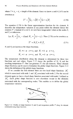
The temperature distribution along the element is determined by these two
functions and end values. Figure 2.12 shows the profiles of Ni, Nj and the
resulting temperature 7". One can generate 7"'s for all elements. These element
shape functions can be used to formulate the global shape functions. Figure 2.13
shows the definition of the global shape functions.
If we consider the first element there are two local shape functions: N:
which is associated with node 1 and Ni associated with node 2. For the second
element again we have a local shape function associated with node 2 defined as
N;. Each global shape function is zero elsewhere except in the elements
associated with the corresponding nodes. This enables us to define the global
temperature variation.

_-_ ---
"d "i
Figure 2.12 Profiles of shape functions N, and Nj and temperature profile T along the element
constructed using shape functions.