Page 114 - Process Modelling and Simulation With Finite Element Methods

Partial Differential Equations and the Finite Element Method 101

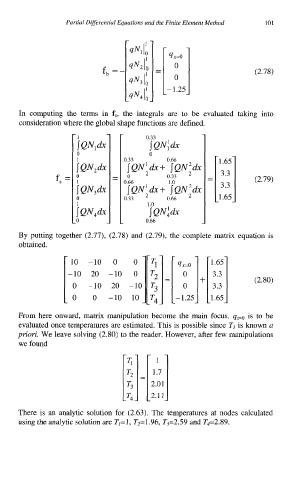
(2.78)

In computing the terms in fs, the integrals are to be evaluated taking into
consideration where the global shape functions are defined,

n
0.33 0.66 1.65
jQN:dx+ [QN2dx
f, = 0.66 0.31 3.3 (2.79)
0
1 .o
jQNidx+ JQN2dx 3.3
0.33 0.66 1.65
L 0.66 -

By putting together (2.77), (2.78) and (2.79), the complete matrix equation is
obtained.

(2.80)

From here onward, matrix manipulation become the main focus. qF0 is to be
i]=[l:71
evaluated once temperatures are estimated. This is possible since TI is known a
priori. We leave solving (2.80) to the reader. However, after few manipulations
we found

2.01

2.11

There is an analytic solution for (2.63). The temperatures at nodes calculated
using the analytic solution are T,=l, T2=1.96, T3=2.59 and T4=2.89.