Page 115 - Process Modelling and Simulation With Finite Element Methods

102 Process Modelling and Simulation with Finite Element Methods

Clearly, four element approximate solutions are not particularly accurate.
The reader can readily implement this example in FEMLAB for arbitrary
accuracy. The purpose of this four element worked example is to make concrete
all the steps that are automatically done by FEMLAB upon specifying the
problem (2.63) and using the default settings and options.
This example discussed the basics of FEM. However we left untouched
many important issues. For an in depth study of FEM the reader is referred to [3]
and [6]. The example is targeted to give an insight to what happens inside
FEMLAB when you set the problem and ask it to solve. The availability of
software packages like FEMLAB greatly reduces the need for understanding the
fundamentals of the FEM. Instead of spending a considerable time on learning
the method, one can concentrate on solving the problems and physics involved.
However, it should be mentioned that an understanding of the core issues in
FEM might help in describing the errors and interpreting solutions in some
cases.

Exercise: Steady state heat transfer in 3-0
In section 2.1.1 we considered the steady state heat transfer equation with a
distributed source, the Poisson equation. Here, we demonstrate the 3-D solution
without the source - Laplace’s equation. There is nothing particularly new in
this example except the demonstration of 3-D modeling. Since all of the models
in this book are run on a relatively low performance PC, complicated 3-D
modeling would tax its resources. Consequently, this is the only 3-D example in
the book. In 3-D modeling it is especially important to conserve memory by
taking full advantage of symmetries in your geometry. In this problem, we will
model the steady heat transfer within a hexagonal prism with differentially
heated (or cooled) basal and side planes. The basal planes are held at the hot
temperature (T=l) and the side faces are held at the cold temperature (T=O).
Since the steady state solution is sought, the thermal diffusivity is immaterial -
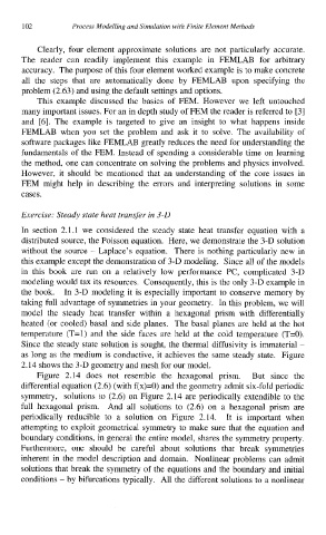
as long as the medium is conductive, it achieves the same steady state. Figure
2.14 shows the 3-D geometry and mesh for our model.
Figure 2.14 does not resemble the hexagonal prism. But since the
differential equation (2.6) (with f(x)=O) and the geometry admit six-fold periodic
symmetry, solutions to (2.6) on Figure 2.14 are periodically extendible to the
full hexagonal prism. And all solutions to (2.6) on a hexagonal prism are
periodically reducible to a solution on Figure 2.14. It is important when
attempting to exploit geometrical symmetry to make sure that the equation and
boundary conditions, in general the entire model, shares the symmetry property.
Furthermore, one should be careful about solutions that break symmetries
inherent in the model description and domain. Nonlinear problems can admit
solutions that break the symmetry of the equations and the boundary and initial
conditions - by bifurcations typically. All the different solutions to a nonlinear