Page 118 - Process Modelling and Simulation With Finite Element Methods

Partial Differential Equations and the Finite Element Method 105

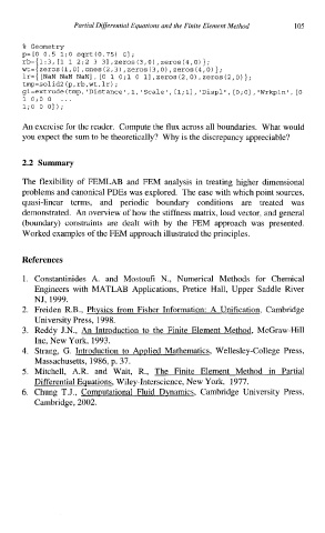
% Geometry
p=[o 0.5 l;O sqrt(0.75) 01;
rb={1:3, [l 1 2;2 3 31 ,zeros(3,0) ,zeros(4,0)};
wt={ zeros (I, 0) ,ones (2,3) ,zeros (3,0) ,zeros (4,0) } ;
lr={ [NaN NaN NaN], [O 1 0;l 0 11 ,zeros(2,0) ,zeros(2,0));
trnp=solid2 (p,rb,wt, lr) ;
gl=extrude(trnp, 'Distance',l, 'Scale', [1;1], 'Displ', [O;O], 'Wrkpln', [O
1o;o 0 ...
l;o 0 01);

An exercise for the reader. Compute the flux across all boundaries. What would
you expect the sum to be theoretically? Why is the discrepancy appreciable?

2.2 Summary

The flexibility of FEMLAB and FEM analysis in treating higher dimensional
problems and canonical PDEs was explored. The ease with which point sources,
quasi-linear terms, and periodic boundary conditions are treated was
demonstrated. An overview of how the stiffness matrix, load vector, and general
(boundary) constraints are dealt with by the FEM approach was presented.
Worked examples of the FEM approach illustrated the principles.

References

1. Constantinides A. and Mostoufi N., Numerical Methods for Chemical
Engineers with MATLAB Applications, Pretice Hall, Upper Saddle River
NJ, 1999.
2. Freiden R.B., Physics from Fisher Information: A Unification, Cambridge
University Press, 1998.
3. Reddy J.N., An Introduction to the Finite Element Method, McGraw-Hill
Inc, New York, 1993.
4. Strang, G. Introduction to Applied Mathematics, Wellesley-College Press,
Massachusetts, 1986, p. 37.
5. Mitchell, A.R. and Wait, R., The Finite Element Method in Partial
Differential Equations, Wiley-Interscience, New York, 1977.
6. Chung T.J., Computational Fluid Dynamics, Cambridge University Press,
Cambridge, 2002.