Page 122 - Process Modelling and Simulation With Finite Element Methods

Multiphysics 109

Here, the dependent variables are described as follows: u is the velocity vector, p
is the pressure, and T is the temperature. The independent variables are spatial
coordinates (implied in the differential operators) and time t. Everything else is
a parameter ( V, p, a, K, g) with fixed value once the fluid and venue are selected.
If there is no imposed moving boundary or pressure gradient, then the whole of
the motion is created by temperature gradients and is termed buoyant (or free)
convection. If there are imposed velocities or pressure gradients, then the
application is termed forced convection. Either case can be studied by the same
multiphysics mode created in FEMLAB, but are historically considered different
physical modes.
In buoyant convection, there are two dimensionless parameters that govern the
dynamical similarity of the problem, the Prandtl number that is a function of the
fluid, and the Rayleigh number that gives the relative importance of temperature
driving forces to dissipative mechanisms:
V
Pr = -
K
ag (V’ (3.2)
Ra =
PVK

where h is the depth of the fluid, 6T is the applied temperature difference, a is
the coefficient of thermal expansion, g is the gravitational acceleration vector (g
is its magnitude), p is the density, v the kinematic viscosity, and K is the thermal
diffusivity .
Batchelor [2] showed that differentially heating any sidewall automatically
induces buoyant motion, so the canonical buoyant convection problem is the hot
walllcold wall cavity flow. This problem is always taken as a test case for the
development of new numerical methods for transport phenomena. We will develop
a FEMLAB model for it in this section. This problem is treated in [3], but the
variations on the theme treated here are original.
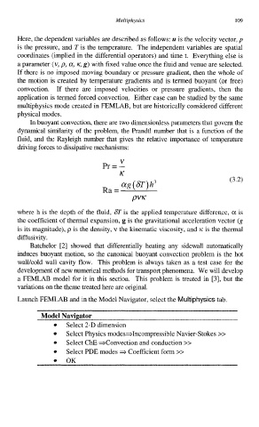
Launch FEMLAB and in the Model Navigator, select the Multiphysics tab.

Model Navigator
Select 2-D dimension
Select Physics modes-Incompressible Navier-Stokes >>
Select ChE =Convection and conduction >>
Select PDE modes 3 Coefficient form >>
OK