Page 123 - Process Modelling and Simulation With Finite Element Methods

110 Process Modelling and Simulation with Finite Element Methods

The last mode, the coefficient form, will be used to solve directly for the
streamfunction from the streamfunction vorticity Poisson equation:

V21y = --LL) (3.3)
You may have noticed that the Incompressible Navier-Stokes application mode
will print “flowlines.” But to my eye, they are streaklines of randomly
positioned particles, rather than the streamlines (contours of streamfunction) that
are traditionally interpreted in two-dimensional flow. Adding equation (3.3) is
straightforward, and not particularly expensive to compute.
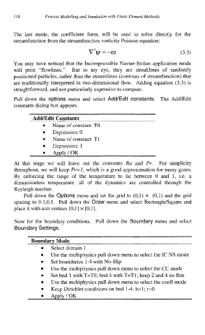
Pull down the options menu and select Add/Edit constants. The AddEdit
constants dialog box appears.
Add/Edit Constants
Name of constant: TO
Expression: 0
Name of constant: T1
Expression: I

At this stage we will leave out the constants Ra and Pr. For simplicity
throughout, we will keep Pr=l, which is a good approximation for many gases.
By enforcing the range of the temperature to lie between 0 and I, i.e. a
dimensionless temperature, all of the dynamics are controlled through the
Rayleigh number.
Pull down the Options menu and set the grid to (0,l) x (0,l) and the grid
spacing to 0.1,O.l. Pull down the Draw menu and select Rectangle/Square and
place it with unit vertices [0,1] x [0,1].

Now for the boundary conditions. Pull down the Boundary menu and select
Boundary Settings.
Boundary Mode
Select domain 1
Use the multiphysics pull down menu to select the IC NS mode
Set boundaries 1-4 with No-Slip
0
Use the multiphysics pull down menu to select the CC mode
0 Set bnd 1 with T=TO; bnd 4 with T=T1; keep 2 and 4 no flux
Use the multiphysics pull down menu to select the coeff mode
Keep Dirichlet conditions on bnd 1-4: h=l; r=O
Apply/OK