Page 128 - Process Modelling and Simulation With Finite Element Methods

Multiphysics 115

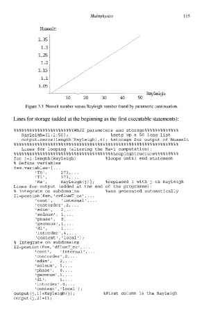
Nusselt

1.35 [
1.3
[
1.25 1
1.2

Figure 3.3 Nusselt number versus Rayleigh number found by parametric continuation.

Lines for storage (added at the beginning as the first executable statements):
%%%%%%%%%%%%%%%%%%%%%%%WBJZ parameters and storage%%%%%%%%%%%%%
Rayleigh= [l : 1 : 501 ; %sets up a 50 long list
output=zeros(length(Rayleigh),4); %storage for output of Nusselt
...............................................................
Lines for looping (altering the Ra=l computation):
%%%%%%%%%%%%%%%%%%%%%%%%%%%%%%%%%%%%%%~oopingstructure%%%%%%%%%
for j=1: length(Ray1eigh) %loops until end statement
% Define variables
fem.variables={ ...
.
'TO', 273,. .
,
'Tl' 373,. . .
,
'Ra' Rayleigh(j) }; %replaces 1 with j-th Rayleigh
Lines for output (added at the end of the programme):
% Integrate on subdomains %was generated automatically
Il=postint(fem,'cvfluxT-cc' ,...
'cont', 'internal', ...
'contorder',2, ...
.
'edim' 2,. .
,
'solnum', 1, ...
'phase', 0, ...
'geomnum' ,1, . .
.
,
'dl' 1, ...
'intorder',4, ...
' context , ' local ) ;
1
% Integrate on subdomains
12=postint(fem,'dfluxT-cc8, ...
'cont', 'internal', ...
'contorder',2, ...
'edim' , 2, . . .
'sohum', 1,. .
.
'phase', 0, ...
'geomnum',l, ...
'dl', 1, ...
lintorder',4, ...
1 context , local ) ;
I
output(j,l)=Rayleigh(j) %First column is the Rayleigh
;
output ( j ,2 ) =I1 ;