Page 130 - Process Modelling and Simulation With Finite Element Methods

Multiphysics 117

Although parametric continuation is therefore possible in the FEMLAB GUI,
it is probably too time consuming to wait for the GUI to process 50 or 100
solutions at a time. So the user will probably want to invest some time in learning
MATLAB programming tools and gaining a handle on the FEMLAB function
library. Fortunately, FEMLAB’s logging feature which records the FEMLAB
commands issued by the GUI provides an excellent starting point for constructing
your own FEMLAB programme. We have already given several applications of
MATLAB programming with FEMLAB functions, but a full description of either
MATLAB programming or FEMLAB functions is beyond the scope of this book.
Chapter one (matrix operations) and the Appendix (vector calculus) provide
only a rudimentary working capacity in MATLAB programming. We will continue
to use this user defined programming style in the book, with sufficient explanation
to guide the informed reader, and at least to inform the MATLAB novice of what
power they are missing out on!
Variations on a Theme: Non-Monotonic Density
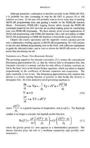
The governing equations for buoyant convection (3.1) assume the conventional
Boussinesq approximation [4], i.e. that the velocity field is divergence free, that
kinematic viscosity is constant, and that the only effects of density variation are
felt by the body force in the Navier-Stokes equations, which was taken to depend
proportionally to the coefficient of thermal expansion and temperature. The
latter constraint, is too severe. The Boussinesq approximation only requires that
density is a slowly varying function of position so that locally the velocity is
divergence free. So a less restrictive set of governing equations is
au
-+u.vu =--Vv13+vV2u+- P m
1
at Po Po

v.u=o (3.6)
dT
-+U.VT = KV’T
at

where - general function of temperature, and po=p(To). The Rayleigh
is
a
Po
number is no longer a constant, but depends on this function:

where the gravity group Gr’ now appears as a dimensionless parameter. The
density function plays the role of a nonlinear expansivity (and possibly non-
monotonic).