Page 127 - Process Modelling and Simulation With Finite Element Methods

114 Process Modelling and Simulation with Finite Element Methods

Contour: temperature 0
F
..
~, ..
.. .
.~ ..
..
i. ... . ....
....

.
%
.. .
.
.. . ...
..
...
. . . &
I I I I I I I I I
0 0.1 0.2 0.3 0.4 0.5 0.6 0.7 0.8 0.9 1
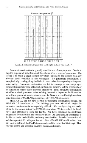
Figure 3.2 Isotherms between 0 (left) and 1 (right) at steady state for Ra=I.

Parametric continuation is typically used for one of two purposes. One is to
map the response of some feature of the solution over a range of parameters. The
second is to reach a target solution for which jumping to the solution from any
arbitrary initial condition is non-convergent. So parametric continuation is
metaphorically crawling along the limb of a tree, rather than expecting to jump and
arrive safely. Parametric continuation can fail to converge as one ramps up a
complexity parameter (like a Rayleigh or Reynolds number), and the complexity of
the solution at smaller scales becomes unresolved. Thus, parametric continuation
identifies at which parameter values refining the mesh is important. In this section,
we will use parametric continuation to map the Nusselt versus Rayleigh numbers,
using the power of MATLAB programming of FEMLAB subroutines.
FEMLAB 2.2 did not have a built in parametric continuation feature, but
FEMLAB 2.3 introduced it. Yet building your own MATLAB m-file for
parametric continuation is not especially difficult. We start by saving the model
M-file for the current state of the FEMLAB simulation. We have solved for Ra=O,
Ra=l, and attempted to solve for Ra=50. We have computed the subdomain
integrations for conductive and convective fluxes. All the FEMLAB commands to
do this are in the model M-file, and many more besides. SaveAs “convection.m”
and then open this file with your favorite editor of MATLAB’s m-file editor. You
will want to delete all the PostPlot commands, and the entire Ra=50 attempt. Then
you will need to add a looping structure, storage, and output.