Page 125 - Process Modelling and Simulation With Finite Element Methods

112 Process Modelling and Simulation with Finite Element Methods

to “resolve” the noise, which is not particularly sensible. Solution - turn the feature
off! Select under Solver Parameters the Scaling box, and in the pop-up
dialogue box, select “none” rather than the default automatic.
The second point about the pressure datum is discussed in detail in Chapter 5.
The solutions here are convergent, but greater accuracy and faster convergence
result by specifying a pressure datum.
To implement a buoyant force that varies with temperature, edit the
appropriate subdomain setting for the IC NS mode to be:
Fy = RaT (3.4)

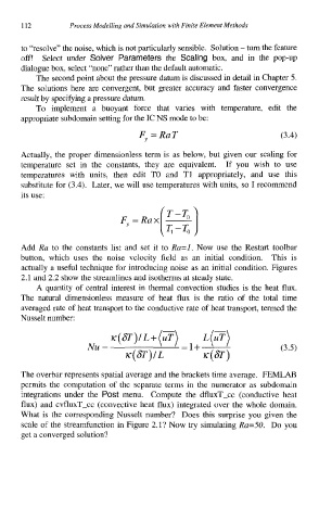
Actually, the proper dimensionless term is as below, but given our scaling for
temperature set in the constants, they are equivalent. If you wish to use
temperatures with units, then edit TO and TI appropriately, and use this
substitute for (3.4). Later, we will use temperatures with units, so I recommend
its use:

Add Ra to the constants list and set it to Ra=l. Now use the Restart toolbar
button, which uses the noise velocity field as an initial condition. This is
actually a useful technique for introducing noise as an initial condition. Figures
2.1 and 2.2 show the streamlines and isotherms at steady state.
A quantity of central interest in thermal convection studies is the heat flux.
The natural dimensionless measure of heat flux is the ratio of the total time
averaged rate of heat transport to the conductive rate of heat transport, termed the
Nusselt number:

(3.5)

The overbar represents spatial average and the brackets time average. FEMLAB
permits the computation of the separate terms in the numerator as subdomain
integrations under the Post menu. Compute the dfluxT-cc (conductive heat
flux) and cvfluxT-cc (convective heat flux) integrated over the whole domain.
What is the corresponding Nusselt number? Does this surprise you given the
scale of the streamfunction in Figure 2.1? Now try simulating Ra=50. Do you
get a converged solution?