Page 124 - Process Modelling and Simulation With Finite Element Methods

Multiphysics 111

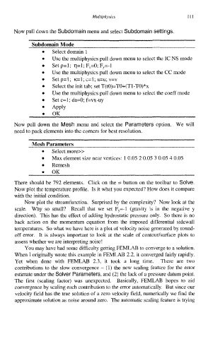
Now pull down the Subdomain menu and select Subdomain settings.

Subdomain Mode
Select domain 1
0 Use the multiphysics pull down menu to select the IC NS mode
0 Set p=l; q=1; F,=O; F,=-l
0 Use the multiphysics pull down menu to select the CC mode
Set p=1; ~=l; c=l; u=u; v=v
Select the init tab; set T(tO)=TO+(Tl-TO)*x
Use the multiphysics pull down menu to select the coeff mode

0 Set c=l; da=O; f=vx-uy
Apply
0 OK
Now pull down the Mesh menu and select the Parameters option. We will
need to pack elements into the corners for best resolution.

Mesh Parameters
Select more>>
Max element size near vertices: 1 0.05 2 0.05 3 0.05 4 0.05
0 Remesh
OK
0
There should be 792 elements. Click on the = button on the toolbar to Solve.
Now plot the temperature profile. Is it what you expected? How does it compare
with the initial condition.
Now plot the streamfunction. Surprised by the complexity? Now look at the
scale. Why so small? Recall that we set F,=-1 (gravity is in the negative y
direction). This has the effect of adding hydrostatic pressure only. So there is no
back action on the momentum equation from the imposed differential sidewall
temperatures. So what we have here is a plot of velocity noise generated by round-
off error. It is always important to look at the scale of contoudsurface plots to
assess whether we are interpreting noise!
You may have had some difficulty getting FEMLAB to converge to a solution.
When I originally wrote this example in FEMLAB 2.2, it converged fairly rapidly.
Yet when done with FEMLAB 2.3, it took a long time. There are two
contributions to the slow convergence - (1) the new scaling feature for the error
estimate under the Solver Parameters, and (2) the lack of a pressure datum point.
The first (scaling factor) was unexpected. Basically, FEMLAB hopes to aid
convergence by scaling each contribution to the error automatically. But since our
velocity field has the true solution of a zero velocity field, numerically we find the
approximate solution as noise around zero. The automatic scaling feature is trying