Page 133 - Process Modelling and Simulation With Finite Element Methods

120 Process Modelling and Simulation with Finite Element Methods
sf=nco-1:-1:l; % Scale factors for differentiation
dco=sf(ones(npy,l),:).*co(:,l:nco-1); % Derivative coefficients
ppd=mkpp (br, dco) ; % Build up pp form for derivative
a=ppval (ppd, tternp) ;
This m-file (dwatrden.m) should also be loaded into your MATLAB current
directory. It uses a MATLAB programming technique to compute the
approximate first derivative of a cubic spline interpolation. Very clever. I wish
I could take credit for it, but that goes to others [5]. It has been pointed out to me
that I re-invented the wheel in that FEMLAB developers recognized the need for
derivatives of interpolated functions, so they introduced their own interpolation
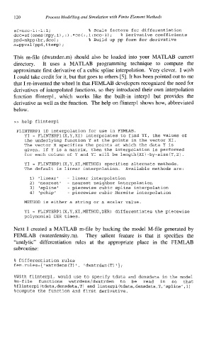
function flinterpl, which works like the built-in interpl but provides the
derivative as well as the function. The help on flinterpl shows how, abbreviated
below.

>> help flinterpl
FLINTERPl 1D interpolation for use in FEMLAB.
YI = FLINTERPl(X,Y,XI) interpolates to find YI, the Values of
the underlying function Y at the points in the vector XI.
The vector X specifies the points at which the data Y is
given. If Y is a matrix, then the interpolation is performed
for each column of Y and YI will be length(XI)-by-size(Y,2).
YI = FLINTERPl(X,Y,XI,METHOD) specifies alternate methods.
The default is linear interpolation. Available methods are:
1) ‘linear’ - linear interpolation
2) ‘nearest’ - nearest neighbor interpolation
3) ‘spline’ - piecewise cubic spline interpolation
4) ’ pchip ’ - piecewise cubic Hermite interpolation
METHOD is either a string or a scalar value
YI = FLINTERPl(X,Y,XI,METHOD,DER) differentiates the piecewise
polynomial DER times.

Next I created a MATLAB m-file by hacking the model M-file generated by
FEMLAB (waterdensity.m). They salient feature is that it specifies the
“analytic” differentiation rules at the appropriate place in the FEMLAB
subroutine:
% Differentiation rules
fem.rules={ ‘watrdens ’
(T) I, ‘dwatrden(T) } ;
%With flinterpl, would use to specify tdata and densdata in the model
%m-file functions watrdens/dwatrden to be read in so that
%flinterpl(tdata,densdata,T) and linterpl(tdata,densdata,T,’spline’,i)
%compute the function and first derivative.