Page 117 - Process Modelling and Simulation With Finite Element Methods

104 Process Modelling and Simulation with Finite Element Methods

Boundary Mode
Select domain 1,2 (sides) and choose Neumann
Select domain 3,4 (top, bottom) and choose Dirichlet
and set h=l, r=l
Select domain 5 (back) and choose Dirichlet and set
h= 1, r=O
OK
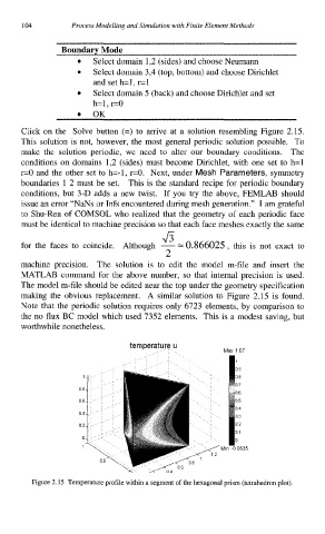
Click on the Solve button (=) to arrive at a solution resembling Figure 2.1.5.
This solution is not, however, the most general periodic solution possible. To
make the solution periodic, we need to alter our boundary conditions. The
conditions on domains 1,2 (sides) must become Dirichlet, with one set to h=l
r=O and the other set to h=-1, r=O. Next, under Mesh Parameters, symmetry
boundaries 1 2 must be set. This is the standard recipe for periodic boundary
conditions, but 3-D adds a new twist. If you try the above, FEMLAB should
issue an error “NaNs or Infs encountered during mesh generation.” I am grateful
to Shu-Ren of COMSOL who realized that the geometry of each periodic face
must be identical to machine precision so that each face meshes exactly the same

for the faces to coincide. Although - =: 0.866025, this is not exact to
2
machine precision. The solution is to edit the model m-file and insert the
MATLAB command for the above number, so that internal precision is used.
The model m-file should be edited near the top under the geometry specification
making the obvious replacement. A similar solution to Figure 2.15 is found.
Note that the periodic solution requires only 6723 elements, by comparison to
the no flux BC model which used 73.52 elements. This is a modest saving, but
worthwhile nonetheless.

temperature u
Max 107

1,
08.
06.
04,
02,
0,
1

Figure 2.15 Temperature profile within a segment of the hexagonal prism (tetrahedron plot)