Page 113 - Process Modelling and Simulation With Finite Element Methods

100 Process Modelling and Simulation with Finite Element Methods

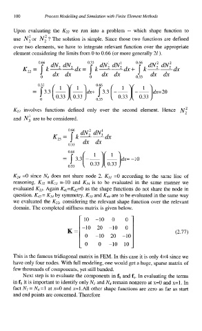
Upon evaluating the Kzz we run into a problem -- which shape function to
use Ni or N; ? The solution is simple. Since those two functions are defined
over two elements, we have to integrate relevant function over the appropriate
element considering the limits from 0 to 0.66 (or more generally 21 ).
0.66 dN, dN2 0.33 dNi dNi dx + '7 dNl dNl
dx
K,, = k-- dx= I k-- --
dx dx 0 dx dx 0.33 dx dx
= 0.33 [ 3.3 [ L][ L]dx+ lE.3 [ -&)[ -&)dx=20

0.33 0.33

K2, involves functions defined only over the second element. Hence Nt
and N: are to be considered.

0.66 dN; dN; dx
K23= k--
0.33 dx dx

= 073,3(-L](+= 0.33 -10
0.33
0.33
K24 =O since N4 does not share node 2. Kjl =O according to the same line of
reasoning. Kj2 =KZ3 =-lo and Kj4 is to be evaluated in the same manner we
evaluated KZ3. Again &1=K42=0 as the shape functions do not share the node in
question. K43 = K34 by symmetry. K33 and K44 are to be evaluated in the same way
we evaluated the Kz2, considering the relevant shape function over the relevant
domain. The completed stiffness matrix is given below.
10 -10 0 0
-10 20 -10 0
(2.77)

This is the famous tridiagonal matrix in FEM. In this case it is only 4x4 since we
have only four nodes. With full modeling, one would get a huge, sparse matrix of
few thousands of components, yet still banded.
Next step is to evaluate the components in fb and f,. In evaluating the terms
in fb it is important to identify only N, and N4 remain nonzero at x=O and x=l . In
fact Nl = N4 =1 at x=O and x=l.All other shape functions are zero as far as start
and end points are concerned. Therefore