Page 112 - Process Modelling and Simulation With Finite Element Methods

Partial Differential Equations and the Finite Element Method 99

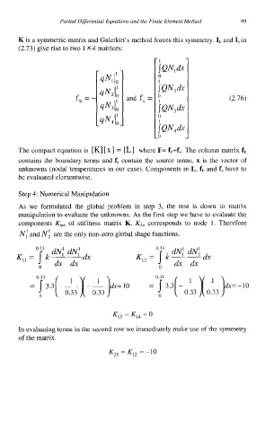
K is a synmetric matrix and Galerkin's method forces this symmetry. Ib and I, in
(2.73) give rise to two 1 X4 matrices:

(2.76)

The compact equation is [K] { x} = { L} where F= fb+f,. The column matrix fb
contains the boundary terms and f, contain the source terms. x is the vector of
unknowns (nodal temperatures in our case). Components in L, fb and f, have to
be evaluated elementwise.

Step 4: Numerical Manipulation
As we formulated the global problem in step 3, the rest is down to matrix
manipulation to evaluate the unknowns. As the first step we have to evaluate the
components K,, of stiffness matrix K. K,, corresponds to node 1. Therefore
N: and Ni are the only non-zero global shape functions.

0.33 dN: dN: dx 0.33 dN: dNk
K,, = k-- K12 = 5 k-- dx
0 dx dx 0 dx dx
0.33
= [ 3.3[-&)[-&&=10

K,, = K,, = 0

In evaluating terms in the second row we immediately make use of the symmetry
of the matrix.