Page 116 - Process Modelling and Simulation With Finite Element Methods

Partial Differential Equations and the Finite Element Method 103

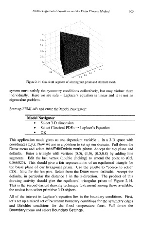
Figure 2.14 One-sixth segment of a hexagonal prism and standard mesh.

system must satisfy the symmetry conditions collectively, but may violate them
individually. Here we are safe - Laplace’s equation is linear and it is not an
eigenvalue problem.

Start up FEMLAB and enter the Model Navigator:
__
Model Navigator
Select 3-D dimension
Select Classical PDEs - Laplace’s Equation
0 OK
This application mode gives us one dependent variable u, in a 3-D space with
coordinates x,y,z. Now we are in a position to set up our domain. Pull down the
Draw menu and select Add/Edit/Delete work plane. Accept the x-y plane and
defaults. Enter a triangle with vertices (O,O), (l,O), (0.5,0.8) by adding line
segments. Edit the last vertex (double clicking) to amend the point to (0.5,
0.866025). This should give a fair representation of an equilateral triangle for
the basal plane of our hexagonal prism. Use the palette to “coerce to solid”
CO1. Now for the fun part. Select from the Draw menu: extrude. Accept the
defaults, in particular the distance 1 in the z-direction. The product of this
drawing activity should give the equilateral triangular prism of Figure 2.14.
This is the second easiest drawing technique (extrusion) among those available;
the easiest is to select primitive 3-D objects.

All of the interest in Laplace’s equation lies in the boundary conditions. First,
let’s set up a mixed set of Neumann boundary conditions for the symmetry edges
and Dirichlet conditions for the fixed temperature faces. Pull down the
Boundary menu and select Boundary Settings.