Page 103 - Process Modelling and Simulation With Finite Element Methods

90 Process Modelling and Simulation with Finite Element Methods

40 60 80 100 120 140
-0.2
Number of elements N
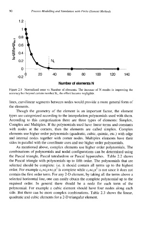
Figure 2.9 Normalized error vs Number of elements. The increase of N results in improving the
accuracy but beyond certain number Nc, the effect become negligible.

lines, curvilinear segments between nodes would provide a more general form of
the elements.
Though the geometry of the element is an important factor, the element
types are categorized according to the interpolation polynomials used with them.
According to this categorization there are three types of elements: Simplex,
Complex and Multiplex. If the polynomials used have linear terms and constants
with nodes at the corners, then the elements are called simplex. Complex
elements use higher order polynomials (quadratic, cubic, quintic, etc.) with edge
and internal nodes together with corner nodes. Multiplex elements have their
sides in parallel with the coordinate axes and use higher order polynomials.
As mentioned above, complex elements use higher order polynomials. The
combinations of polynomials and nodal configurations can be determined using
the Pascal triangle, Pascal tetrahedron or Pascal hypercubes. Table 2.2 shows
the Pascal triangle with polynomials up to fifth order. The polynomials that are
selected should be complete: i.e. it should contain all terms up to the highest
order. For example cI+c2x+c3x2 is complete while c1+c2x2 is not since it does not
contain the first order term. For any 2-D element, by taking all the terms above a
selected horizontal line, one can easily obtain the complete polynomial up to the
required order. In general there should be a node for each term of the
polynomial. For example a cubic element should have four nodes along each
side. But there can be more complex combinations. Table 2.3 shows the linear,
quadratic and cubic elements for a 2-D triangular element.