Page 270 -

252 9 Operational Support

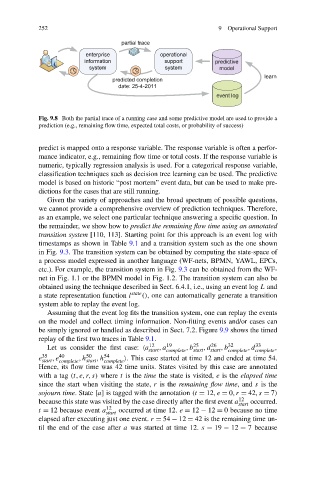
Fig. 9.8 Both the partial trace of a running case and some predictive model are used to provide a
prediction (e.g., remaining flow time, expected total costs, or probability of success)

predict is mapped onto a response variable. The response variable is often a perfor-
mance indicator, e.g., remaining flow time or total costs. If the response variable is
numeric, typically regression analysis is used. For a categorical response variable,
classification techniques such as decision tree learning can be used. The predictive
model is based on historic “post mortem” event data, but can be used to make pre-
dictions for the cases that are still running.
Given the variety of approaches and the broad spectrum of possible questions,
we cannot provide a comprehensive overview of prediction techniques. Therefore,
as an example, we select one particular technique answering a specific question. In
the remainder, we show how to predict the remaining flow time using an annotated
transition system [110, 113]. Starting point for this approach is an event log with
timestamps as shown in Table 9.1 and a transition system such as the one shown
in Fig. 9.3. The transition system can be obtained by computing the state-space of
a process model expressed in another language (WF-nets, BPMN, YAWL, EPCs,
etc.). For example, the transition system in Fig. 9.3 can be obtained from the WF-
net in Fig. 1.1 or the BPMN model in Fig. 1.2. The transition system can also be
obtained using the technique described in Sect. 6.4.1, i.e., using an event log L and
a state representation function l state (), one can automatically generate a transition
system able to replay the event log.
Assuming that the event log fits the transition system, one can replay the events
on the model and collect timing information. Non-fitting events and/or cases can
be simply ignored or handled as described in Sect. 7.2. Figure 9.9 shows the timed
replay of the first two traces in Table 9.1.
Let us consider the first case: a 12 ,a 19 ,b 25 ,d 26 ,b 32 ,d 33 ,
start complete start start complete complete
e 35 ,e 40 ,h 50 ,h 54 . This case started at time 12 and ended at time 54.
start
start
complete
complete
Hence, its flow time was 42 time units. States visited by this case are annotated
with a tag (t,e,r,s) where t is the time the state is visited, e is the elapsed time
since the start when visiting the state, r is the remaining flow time, and s is the
sojourn time. State [a] is tagged with the annotation (t = 12,e = 0,r = 42,s = 7)
12
because this state was visited by the case directly after the first event a start occurred.
t = 12 because event a 12 occurred at time 12. e = 12 − 12 = 0 because no time
start
elapsed after executing just one event. r = 54 − 12 = 42 is the remaining time un-
til the end of the case after a was started at time 12. s = 19 − 12 = 7 because