Page 47 - Rapid Learning in Robotics

3.4 Approximation Types 33

RBF

RBF
norm.

σ < σ < σ
1 2 3

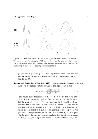
Figure 3.2: Two RBF units constitute the approximation model of a function.
The upper row displays the plain RBF approach versus the results of the normal-
ization step in the lower row.From left to right three basis radii illustrate the
smoothing impact of an increasing to distance ratio.

polynomial regression splines - but only for one or two components
of x (MARS algorithm (“Multivariate Adaptive Regression Splines”;
Friedman 1991).

Normalized Radial Basis Function (RBF) networks take the form of a weighted
sum over reference points w i located in the input space at w i :

P

F w x i jx u i j w i (3.6)
P jx u i j
i

I
The radial basis functions R IR usually decays to zero
with growing argument and is often represented by the Gaussian
p

bell function r e
r , characterized by the width (there-
fore the RBF is sometimes called a kernel function). The division by
the unweighted sum takes care on normalization and flat extrapo-
lation as illustrated in Fig. 3.2. The learning is often split in two
phases: (i) the placement of the centers is learned by an unsuper-
vised method, for example by k-means clustering, learning vector quan-
tization (LVQ2), or competitive learning; (ii) the width is set, often