Page 213 -

196 Computed-Torque Control

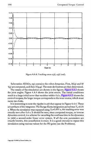
Figure 4.4.4: Tracking error e 1 (t), e 2 (t) (red).

Subroutine ARM(x, xp) contains the robot dynamics. First, M(q) and M -
1 (q) are computed, and then N(q,q). The state derivatives are then determined.
The results of the simulation are shown in the figures. Figure 4.4.3 shows
the joint angles. Figure 4.4.4 shows the joint errors. The initial conditions
result in a large initial error that vanishes within 0.6 s. Figure 4.4.5 shows the
control torques; the larger torque corresponds to the inner motor, which must
move two links.
It is interesting to note the ripples in e(t) that appear in Figure 4.4.4. These
are artifacts of the integrator. The Runge-Kutta integration period was T R=0.01
s. When the simulation was repeated using T R=0.001 s, the tracking error was
exactly zero after 0.6 s. It should be zero, since computed-torque, or inverse
dynamics control, is a scheme for canceling the nonlinearities in the dynamics
to yield a second-order linear error system. If all the arm parameters are
exactly known, this cancellation is exact. It is a good exercise to repeat this
simulation using various values for the PD gains (see the Problems).

Copyright © 2004 by Marcel Dekker, Inc.