Page 39 - Rock Mechanics For Underground Mining

STRESS TRANSFORMATION

equilibrium requirement for the x direction, for example, yields

t x A − xx A x − xy A y − zx A z = 0 (2.6)

or

t x = xx x + xy y + zx z

Equation 2.6 represents an important relation between the traction component, the
state of stress, and the orientation of a surface through the point. Developing the
equilibrium equations, similar to equation 2.6, for the y and z directions, pro-
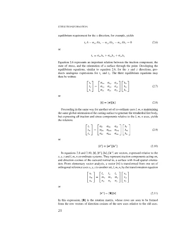
duces analogous expressions for t y and t z . The three equilibrium equations may
then be written
⎡ ⎤ ⎡ ⎤ ⎡ ⎤
t x xx xy zx x
= yy yz ⎦
⎣ t y ⎣ xy ⎦ ⎣ y (2.7)
⎦
t z zx yz zz z
or
[t] = [ ][ ] (2.8)

Proceeding in the same way for another set of co-ordinate axes l, m, n maintaining
the same global orientation of the cutting surface to generate the tetrahedral free body,
but expressing all traction and stress components relative to the l, m, n axes, yields
the relations
⎡ ⎤ ⎡ ⎤ ⎡ ⎤
t l ll lm nl l
⎣ t m ⎦ = ⎣ lm mm mn ⎦ ⎣ m ⎦ (2.9)
t n nl mn nn n
or
[t ] = [ ][ ] (2.10)
∗
∗
∗
∗
∗
In equations 2.8 and 2.10, [t], [t ], [ ], [ ] are vectors, expressed relative to the
x, y, z and l, m, n co-ordinate systems. They represent traction components acting on,
and direction cosines of the outward normal to, a surface with fixed spatial orienta-
tion. From elementary vector analysis, a vector [v] is transformed from one set of
orthogonal reference axes x, y, z to another set, l, m, n, by the transformation equation
⎡ ⎤ ⎡ ⎤ ⎡ ⎤
v l l x l y l z v x
= m y m z ⎦
⎣ v m ⎣ m x ⎦ ⎣ v y
⎦
v n n x n y n z v z
or
∗
[v ] = [R][v] (2.11)
In this expression, [R] is the rotation matrix, whose rows are seen to be formed
from the row vectors of direction cosines of the new axes relative to the old axes.
21