Page 170 - Schaum's Outline of Differential Equations

CHAP. 17] REDUCTION OF LINEAR DIFFERENTIAL EQUATIONS 153

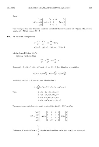
We set

Then the original third-order differential equation is equivalent to the matrix equation x(t) = A(t)x(t) + f(t), or, more
simply, x(0 = A(t)x(t) because f(f) = 0.

17.6. Put the initial-value problem

into the form of System (17.7).
Following Step 1, we obtain

2 2
Hence; a 3(t) = 0, a 2(t) = e', a^t) = -t e ', a 0(t) = 0, and/(f) = 5. If we define four new variables,

we obtain x 1 = x 2, x 2 = x 3, x 3 = x 4, and, upon following Step 3,

Thus,

These equations are equivalent to the matrix equation x(t) = A(t)x(t) + f(t) if we define

Furthermore, if we also define c = then the initial conditions can be given by x(t 0) = c, where t 0=l.