Page 177 - Schaum's Outline of Differential Equations

160 GRAPHICAL METHODS FOR SOLVING DIFFERENTIAL EQUATIONS [CHAP. 18

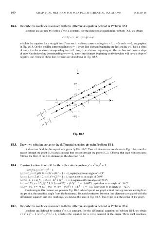
18.2. Describe the isoclines associated with the differential equation defined in Problem 18.1.
Isoclines are defined by setting / = c, a constant. For the differential equation in Problem 18.1, we obtain

which is the equation for a straight line. Three such isoclines, corresponding to c = 1, c = 0, and c = —1, are graphed
in Fig. 18-3. On the isocline corresponding to c = 1, every line element beginning on the isocline will have a slope
of unity. On the isocline corresponding to c = 0, every line element beginning on the isocline will have a slope
of zero. On the isocline corresponding to c = -1, every line element beginning on the isocline will have a slope of
negative one. Some of these line elements are also drawn in Fig. 18-3.

Fig. 18-3

18.3. Draw two solution curves to the differential equation given in Problem 18.1.
A direction field for this equation is given by Fig. 18-2. Two solution curves are shown in Fig. 18-4, one that
passes through the point (0, 0) and a second that passes through the point (0, 2). Observe that each solution curve
follows the flow of the line elements in the direction field.

2
2
18.4. Construct a direction field for the differential equation / = x + y - 1.
2
2
Here/(X y) = x + y - 1.
2
2
Atx = 0,y = 0, /(O, 0) = (O) + (O) - 1 = -1, equivalent to an angle of -45°.
2
2
Atx = 1, ;y = 2,/(l,2) = (l) + (2) - 1=4, equivalent to an angle of 76.0°.
2
2
Atx = -l,y = 2,f(-l, 2) = (-1) + (2) - 1=4, equivalent to an angle of 76.0°.
2
2
At x = 0.25, y = 0.5, f (0.25, 0.5) = (0.25) + (0.5) - 1 = -0.6875, equivalent to an angle of -34.5°.
2
2
At x = -0.3, y = -0.1, /(-0.3, -0.1) = (-0.3) + (-0.1) - 1 = -0.9, equivalent to an angle of -42.0°.
Continuing in this manner, we generate Fig. 18-5. At each point, we graph a short line segment emanating from
the point at the specified angle from the horizontal. To avoid confusion between line elements associated with the
differential equation and axis markings, we deleted the axes in Fig. 18-5. The origin is at the center of the graph.
18.5. Describe the isoclines associated with the differential equation defined in Problem 18.4.
Isoclines are defined by setting y' = c, a constant. For the differential equation in Problem 18.4, we obtain
2
2
2
c = x + y 2 — 1 or x + y = c+ 1, which is the equation for a circle centered at the origin. Three such isoclines,