Page 180 - Schaum's Outline of Differential Equations

CHAP. 18] GRAPHICAL METHODS FOR SOLVING DIFFERENTIAL EQUATIONS 163

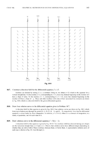
Fig. 18-8

18.7. Construct a direction field for the differential equation / = x!2.
Isoclines are defined by setting y' = c, a constant. Doing so, we obtain x = 2c which is the equation for a
vertical straight line. On the isocline x = 2, corresponding to c = 1, every line element beginning on the isocline will
have a slope of unity. On the isocline x = —\, corresponding to c = —1/2, every line element beginning on the
isocline will have a slope of —I. These and other isoclines with some of their associated line elements are drawn
in Fig. 18-8, which is a direction field for the given differential equation.

18.8. Draw four solution curves to the differential equation given in Problem 18.7.
A direction field for this equation is given by Fig. 18-8. Four solution curves are drawn in Fig. 18-9, which
from top to bottom pass through the points (0, 1), (0, 0), (0, -1), and (0, -2), respectively. Note that the differential
2
equation is solved easily by direct integration. Its solution, y = x /4 + k, where k is a constant of integration, is a
family of parabolas, one for each value of k.

18.9. Draw solution curves to the differential equation y' = 5y(y - I).
A direction field for this equation is given by Fig. 18-10. Two isoclines with line elements having zero slopes
are the horizontal straight lines y = 0 and y=l. Observe that solution curves have different shapes depending on
whether they are above both of these isoclines, between them, or below them. A representative solution curve of
each type is drawn in Fig. 18-ll(a) through (c).