Page 195 - Schaum's Outline of Differential Equations

178 NUMERICAL METHODS FOR SOLVING DIFFERENTIAL EQUATIONS [CHAP. 19

STARTING VALUES
The Adams-Bashforth-Moulton method and Milne's method require information at y 0, y lt y 2, and y 3 to
start. The first of these values is given by the initial condition in Eq. (19.1). The other three starting values are
gotten by the Runge-Kutta method.

ORDER OF A NUMERICAL METHOD

A numerical method is of order n, where n is a positive integer, if the method is exact for polynomials of
degree n or less. In other words, if the true solution of an initial-value problem is a polynomial of degree n or
less, then the approximate solution and the true solution will be identical for a method of order n.
In general, the higher the order, the more accurate the method. Euler's method, Eq. (18.4), is of order one,
the modified Euler's method, Eq. (19.4), is of order two, while the other three, Eqs. (19.5) through (19.7), are
fourth-order methods.

Solved Problems

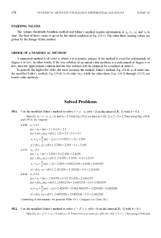
19.1. Use the modified Euler's method to solve y' = y —x; y(0) = 2 on the interval [0, 1] with h = 0.1.
Here/(jt, y) = y -x, x a = 0, and y a = 2. From Eq. (19.2) we have y' Q =/(0, 2) = 2-0 = 2. Then using Eqs. (19.4)
and (19.3), we compute

Continuing in this manner, we generate Table 19-1. Compare it to Table 18-1.

2
19.2. Use the modified Euler's method to solve / = y + 1; y(0) = 0 on the interval [0, 1] with h = 0.1.
2
2
Here/(jt, y) = y + 1, x 0 = 0, and y 0 = 0. From (19.2) we have y^ =/(0, 0) = (O) +1 = 1. Then using (19.4) and