
Page 280 - Schaum's Outline of Differential Equations
P. 280
CHAP. 27] LINEAR DIFFERENTIAL EQUATIONS WITH VARIABLE COEFFICIENTS 263
SOLUTIONS AROUND THE ORIGIN OF HOMOGENEOUS EQUATIONS
Equation (27.7) is homogeneous when g (x) = 0, in which case Eq. (27.2) specializes to
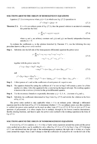
Theorem 27.1. If x = 0 is an ordinary point of Eq. (27.3), then the general solution in an interval containing
this point has the form
where a 0 and a^ are arbitrary constants and Ji(x) and y 2(x) are linearly independent functions
analytic at x = 0.
To evaluate the coefficients a n in the solution furnished by Theorem 27.1, use the following five-step
procedure known as the power series method.
Step 1. Substitute into the left side of the homogeneous differential equation the power series
together with the power series for
and
Step 2. Collect powers of x and set the coefficients of each power of x equal to zero.
Step 3. The equation obtained by setting the coefficient of x" to zero in Step 2 will contain - terms for a finite
a ;
a- term having the largest subscript. The resulting equation
number of j values. Solve this equation for the ;
is known as the recurrence formula for the given differential equation.
Step 4. Use the recurrence formula to sequentially determine a, (j = 2, 3, 4,...) in terms of a 0 and a^.
Step 5. Substitute the coefficients determined in Step 4 into Eq. (27.5) and rewrite the solution in the form
ofEq. (27.4).
The power series method is only applicable when x = 0 is an ordinary point. Although a differential
equation must be in the form of Eq. (27.2) to determine whether x' = 0 is an ordinary point, once this condition
is verified, the power series method can be used on either form (27.7) or (27.2). If P(x) or Q(x) in (27.2) are
quotients of polynomials, it is often simpler first to multiply through by the lowest common denominator,
thereby clearing fractions, and then to apply the power series method to the resulting equation in the form of
Eq. (27.7).
SOLUTIONS AROUND THE ORIGIN OF NONHOMOGENEOUS EQUATIONS
If (f> (x) in Eq. (27.2) is analytic at x = 0, it has a Taylor series expansion around that point and the power
series method given above can be modified to solve either Eq. (27.7) or (27.2). In Step 1, Eqs. (27.5) through
(27.7) are substituted into the left side of the nonhomogeneous equation; the right side is written as a Taylor
series around the origin. Steps 2 and 3 change so that the coefficients of each power of x on the left side of the