Page 221 - Schaum's Outlines - Probability, Random Variables And Random Processes

ANALYSIS AND PROCESSING OF RANDOM PROCESSES [CHAP 6

-4TI-b
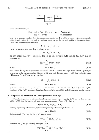
System

Fig. 6-1

linear operator satisfying
T{xl + x,} = Tx, + Tx, = y, + y2 (Additivity)
T{ax} = aTx = ay (Homogeneity)
where a is a scalar number, then the system represented by T is called a linear system. A system is
called time-invariant if a time shift in the input signal causes the same time shift in the output signal.
Thus, for a continuous-time system,

for any value of to, and for a discrete-time system,

for any integer no. For a continuous-time linear time-invariant (LTI) system, Eq. (6.49) can be
expressed as

is known as the impulse response of a continuous-time LTI system. The right-hand side of Eq. (6.50) is
commonly called the convolution integral of h(t) and x(t), denoted by h(t) * x(t). For a discrete-time
LTI system, Eq. (6.49) can be expressed as

where
is known as the impulse response (or unit sample response) of a discrete-time LTI system. The right-
hand side of Eq. (6.52) is commonly called the convolution sum of h(n) and x(n), denoted by h(n) * x(n).

B. Response of a Continuous-Time Linear System to Random Input:
When the input to a continuous-time linear system represented by Eq. (6.49) is a random process
{X(t), t E T,}, then the output will also be a random process {Y(t), t E Ty); that is,

For any input sample function xi(t), the corresponding output sample function is

If the system is LTI, then by Eq. (6.50), we can write

Y(t) = J::(l)X(t - 4 di

Note that Eq. (6.56) is a stochastic integral. Then