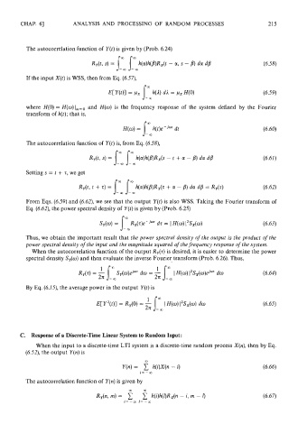
Page 222 - Schaum's Outlines - Probability, Random Variables And Random Processes

CHAP. 61 ANALYSIS AND PROCESSING OF RANDOM PROCESSES

The autocorrelation function of Y(t) is given by (Prob. 6.24)

If the input X(t) is WSS, then from Eq. (6.57),

where H(0) = H(o)I,=, and H(o) is the frequency response of the system defined by the Fourier
transform of h(t); that is,

The autocorrelation function of Y(t) is, from Eq. (6.58),

Setting s = t + z, we get

From Eqs. (6.59) and (6.62), we see that the output Y(t) is also WSS. Taking the Fourier transform of
Eq. (6.62), the power spectral density of Y(t) is given by (Prob. 6.25)

Thus, we obtain the important result that the power spectral density of the output is the product of the
power spectral density of the input and the magnitude squared of the frequency response of the system.
When the autocorrelation function of the output Ry(z) is desired, it is easier to determine the power
spectral density S,(o) and then evaluate the inverse Fourier transform (Prob. 6.26). Thus,

By Eq. (6.15), the average power in the output Y(t) is

C. Response of a Discrete-Time Linear System to Random Input:
When the input to a discrete-time LTI system is a discrete-time random process X(n), then by Eq.
(6.52), the output Y(n) is

The autocorrelation function of Y(n) is given by