Page 268 - Schaum's Outlines - Probability, Random Variables And Random Processes

CHAP. 71 ESTIMATION THEORY

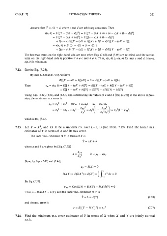
Assume that P = cX + d, where c and d are arbitrary constants. Then
e(c, d) = E{[Y - (cX + d)I2) = E{[Y - (ax + b) + (a - c)X + (b - d)I2)
= E{[Y - (ax + b)I2} + E{[(a - c)X + (b - d)] 2,
+ 2(a - c)E{[ Y - (ax + b)]X) + 2(b - d)E{[Y - (ax + b)]}
= e(a, b) + E{[(a - c)X + (b - d)I2)
+ 2(a - c)E([Y - (ax + b)]X) + 2(b - d)E{[Y - (ax + b)])
The last two terms on the right-hand side are zero when Eqs. (7.68) and (7.69) are satisfied, and the second
term on the right-hand side is positive if a # c and b # d. Thus, e(c, d) 2 e(a, b) for any c and d. Hence,
e(a, b) is minimum.

7.22. Derive Eq. (7.23).
By Eqs. (7.68) and (7.69), we have
R([Y - (ax + b)]aX) = 0 = E([Y - (ax + b)]b)
Then em = e(a, b) = E{[Y - (ax + b)12) = E([Y - (ax + b)][Y - (ax + b)])
= E([Y - (ax + b)]Y) = E(Y2) - aE(XY) - bE(Y)
Using Eqs. (2.31), (3.51), and (3.53), and substituting the values of a and b [Eq. (7.2211 in the above expres-
sion, the minimum m.s. error is

which is Eq. (7.23).

7.23. Let Y = X2, and let X be a uniform r.v. over (- 1, 1) (see Prob. 7.19). Find the linear m.s.
estimator of Y in terms of X and its m.s. error.
The linear m.s. estimator of Y in terms of X is
P=ax+b
where a and b are given by [Eq. (7.2211

Now, by Eqs. (2.46) and (2.44),
px = E(X) = 0

By Eq. (3.51),
ax, = Cov(XY) = E(XY) - E(X)E(Y) = 0
Thus, a = 0 and b = E(Y), and the linear m.s. estimator of Y is
P=b= E(Y)

and the m.s. error is
e = E([Y - E(Y)12) = ay2

7.24. Find the minimum m.s. error estimator of Y in terms of X when X and Y are jointly normal
r.v.'s.