Page 148 - Semiconductor For Micro- and Nanotechnology An Introduction For Engineers

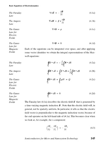
Basic Equations of Electrodynamics
The Faraday
t ∂
Law ∇× E = – ∂B (4.1a)
∂D
The Ampere ∇× H = J + t ∂ (4.1b)
Law
The Gauss ∇• D = ρ (4.1c)
Law for
Electric
Fields

The Gauss ∇• B = 0 (4.1d)
Law for
Magnetic Each of the equations can be integrated over space, and after applying
Fields some vector identities we obtain the integral representations of the Max-
well equations:

∫
•
•
The Faraday ° E dl = – ∂ t ∂ ∫ B d S (4.2a)
Law C S
∫
•
•
•
The Ampere ° H dl = ∫ J d + ∂ t ∂ ∫ D d S (4.2b)
S
Law C S S
•
°
d
The Gauss ∫ D d S = ∫ qV = Q (4.2c)
Law for S V
Electric
Fields
∫
•
The Gauss ° B d S = 0 (4.2d)
Law for S
Magnetic
E
Fields The Faraday law (4.1a) describes the electric field that is generated by
B
a time-varying magnetic induction . Note that the electric field will, in
general, not be spatially uniform. In particular, it tells us that the electric
field vector is perpendicular to the magnetic induction vector, because of
the curl operator on the left-hand side of (4.1a). This becomes clear when
we look at, for example, the x-component:
 ∂E z – ∂E y = – ∂B x (4.3)
∂  y z ∂  t ∂

Semiconductors for Micro and Nanosystem Technology 145