Page 151 - Semiconductor For Micro- and Nanotechnology An Introduction For Engineers

The Electromagnetic System
Box 4.1. The Finite Difference Time-Domain Method.
To solve the Maxwell equations in the time plest FD update formula is accurate to second
domain, computer programs are used that dis- order in space and time.) The Yee cell also guaran-
cretize the space and time coordinates, most fre- tees that the Faraday and Ampere laws are auto-
quently using the finite difference (FD) method. In matically satisfied at each point in the grid through
1966, K. S. Yee [4.2] invented a discretization the update formulas. The two exemplary equations
scheme that still dominates the field, for he was below correspond to the Yee-cell loops in Figure
able to satisfy exactly all the Maxwell equations in B4.1.2:
one swoop, at the same time obtaining a numeri-
cally stable scheme for the explicit time integra-
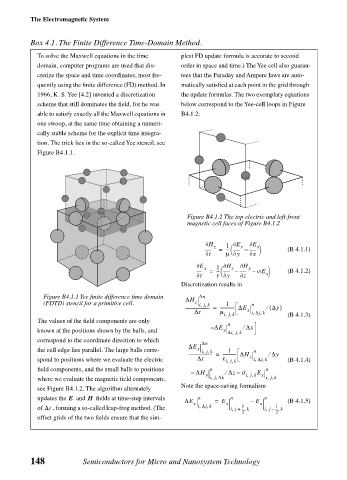
tion. The trick lies in the so-called Yee stencil, see
Figure B4.1.1.

Figure B4.1.2 The top electric and left-front
magnetic cell faces of Figure B4.1.2

∂H z = --- 1 ∂E x – ∂E y (B 4.1.1)

t ∂ µ ∂  y ∂ x 
∂E x 1 ∂H z ∂H y 

t ∂ = --- ε ∂  y – z ∂ – σE x  (B 4.1.2)
Discretization results in
Figure B4.1.1 Yee finite difference time domain ∆H ∆n
(FDTD) stencil for a primitive cell. z ij k 1 n
,,
---------------------- = ------------- ∆E ( ⁄ ∆y)
∆t µ ij k x i ∆jk (B 4.1.3)
,
,
,,
The values of the field components are only n
– ∆E ⁄ ∆x
known at the positions shown by the balls, and y ∆ij k
,,
correspond to the coordinate direction to which ∆n
∆E
the cell edge lies parallel. The large balls corre- x ij k 1 n
,,
---------------------- = ------------ ∆H ⁄ ∆y
,
,
spond to positions where we evaluate the electric ∆t ε ij k z i ∆jk (B 4.1.4)
,,
field components, and the small balls to positions n n
–
– ∆H y ⁄ ∆z σ ij k E x
,,
,,
,,
where we evaluate the magnetic field components, ij ∆k ij k
Note the space-saving formalism
see Figure B4.1.2. The algorithm alternately
updates the E and H fields at time-step intervals n n n
∆E x = E x – E x (B 4.1.5)
,
,
of ∆t , forming a so-called leap-frog method. (The i ∆jk ij +, 1 --- k ij –, 1 --- k
,
,
2 2
offset grids of the two fields ensure that the sim-
148 Semiconductors for Micro and Nanosystem Technology