Page 205 - Semiconductor For Micro- and Nanotechnology An Introduction For Engineers

Transport Theory
tribution at least locally in space. In addition we assume that the scatter-
ing term may be written as
,,
(
,,
f kx t) – f ( kx t)
0
,,
(
(
–
1
Cf kx t)) = – ------------------------------------------------------ = τ δ f kx t,,( , ) (6.23)
τ
i.e., a rate τ – 1 multiplied by the deviation δ f kx t,,( ) of the actual distri-
,,
bution function f kx t,,( ) from its equilibrium value f ( kx t) , see
0
Figure 6.3.
v y
Equilibrium
distribution Drift velocity
f ( kx t)
,,
0
v x
v
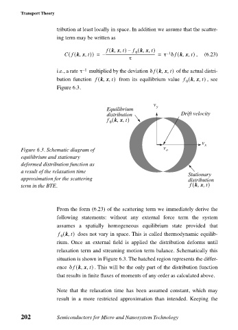
Figure 6.3. Schematic diagram of o
equilibrium and stationary
deformed distribution function as
a result of the relaxation time
Stationary
approximation for the scattering distribution
,,
(
term in the BTE. f kx t)
From the form (6.23) of the scattering term we immediately derive the
following statements: without any external force term the system
assumes a spatially homogeneous equilibrium state provided that
,
f ( k t) does not vary in space. This is called thermodynamic equilib-
0
rium. Once an external field is applied the distribution deforms until
relaxation term and streaming motion term balance. Schematically this
situation is shown in Figure 6.3. The hatched region represents the differ-
ence δ f kx t,,( ) . This will be the only part of the distribution function
that results in finite fluxes of moments of any order as calculated above.

Note that the relaxation time has been assumed constant, which may
result in a more restricted approximation than intended. Keeping the

202 Semiconductors for Micro and Nanosystem Technology