Page 132 - Sensing, Intelligence, Motion : How Robots and Humans Move in an Unstructured World

VISION AND MOTION PLANNING 107

reached physically. In algorithms with vision a hit point may be defined from
a distance, thanks to the robot’s vision, and the robot will not necessarily pass
through this location. For a path segment whose point T i moves along an obstacle
boundary, the firstly defined T i that lies on the M-line is a special point called
the leave point, L. Again, the robot may or may not pass physically through that
point. As we will see, the main difference between the two algorithms VisBug-21
and VisBug-22 is in how they define intermediate targets T i . Their resulting paths
will likely be quite different. Naturally, the current T i is always at a distance from
the robot no more than r v .
While scanning its field of vision, the robot may be detecting some contiguous
sets of visible points—for example, a segment of the obstacle boundary. A point
Q is contiguous to another point S over the set {P }, if three conditions are
met: (i) S ∈{P }, (ii) Q and {P } are visible, and (iii) Q can be continuously
connected with S using only points of {P }.A set is contiguous if any pair of its
points are contiguous to each other over the set. We will see that no memorization
of contiguous sets will be needed; that is, while “watching” a contiguous set, the
robot’s only concern will be whether two points that it is currently interested in
are contiguous to each other.
A local direction is a once-and-for-all determined direction for passing around
an obstacle; facing the obstacle, it can be either left or right. Because of incom-
plete information, neither local direction can be judged better than the other. For
the sake of clarity, assume the local direction is always left.
The M-line divides the environment into two half-planes. The half-plane that
lies to the local direction’s side of M-line is called the main semiplane.The
other half-plane is called the secondary semiplane. Thus, with the local direction
“left,” the left half-plane when looking from S toward T is the main semiplane.
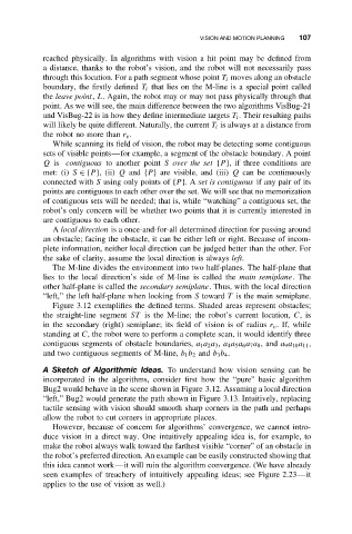
Figure 3.12 exemplifies the defined terms. Shaded areas represent obstacles;
the straight-line segment ST is the M-line; the robot’s current location, C,is
in the secondary (right) semiplane; its field of vision is of radius r v . If, while
standing at C, the robot were to perform a complete scan, it would identify three
contiguous segments of obstacle boundaries, a 1 a 2 a 3 , a 4 a 5 a 6 a 7 a 8 ,and a 9 a 10 a 11 ,
and two contiguous segments of M-line, b 1 b 2 and b 3 b 4 .

A Sketch of Algorithmic Ideas. To understand how vision sensing can be
incorporated in the algorithms, consider first how the “pure” basic algorithm
Bug2 would behave in the scene shown in Figure 3.12. Assuming a local direction
“left,” Bug2 would generate the path shown in Figure 3.13. Intuitively, replacing
tactile sensing with vision should smooth sharp corners in the path and perhaps
allow the robot to cut corners in appropriate places.
However, because of concern for algorithms’ convergence, we cannot intro-
duce vision in a direct way. One intuitively appealing idea is, for example, to
make the robot always walk toward the farthest visible “corner” of an obstacle in
the robot’s preferred direction. An example can be easily constructed showing that
this idea cannot work—it will ruin the algorithm convergence. (We have already
seen examples of treachery of intuitively appealing ideas; see Figure 2.23—it
applies to the use of vision as well.)