Page 293 - Sensing, Intelligence, Motion : How Robots and Humans Move in an Unstructured World

268 MOTION PLANNING FOR TWO-DIMENSIONAL ARM MANIPULATORS

obstacle O that lies fully in the arm workspace, as shown. Obstacle O is a
square with the side length l/4.
Recall that the method of motion planning with complete information (Piano
Mover’s model) [13] requires one to first approximate the configuration space
(C-space) image of obstacle O by a polygon. Call the obstacle in C-space
O C and call the approximating polygon P C .Let δ be the maximum linear
deviation of P C from O C . Evaluate the minimum order (the number of sides)
of the polygon P C that will keep δ within 1% of the perimeter of P C .
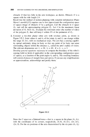
2. Consider a two-link planar robot arm with revolute joints, as shown in
Figure 5.E.2. Joint values θ 1 and θ 2 of the joints J 0 and J 1 can change within
the range (0, 2π), with no mechanical stops. The arm has a sensing capabil-
ity spread uniformly along its body so that any point of its body can sense
surrounding objects within the distance r v , called the arm’s radius of vision.
The relevant dimensions are: l 1 = 30,l 2 = 20,R = 2,r v = 3.
Develop general equations necessary to compute the boundary of the robot’s
sensing field (or fields if applicable) in the corresponding configuration space
(C-space), as a function of the joint angles θ 1 and θ 2 . The resulting boundary
will consist of pieces of straight lines and curves. If you use any simplifications
or approximations, acknowledge and justify them.

R

b

r v
Θ 2
l 2

a
J 1
l 1

Θ 1

J o

Figure 5.E.2

Draw the C-space as a flattened torus—that is, a square in the plane (θ 1 ,θ 2 ),
with the coordinates of its corners, respectively, (0, 0), (0, 2π), (2π, 2π),
(2π, 0). For the six positions of the arm characterized by the six pairs (θ 1 ,θ 2 )